Least Squares Regression Method
Vitalnet uses the "least squares" regression method to determine the time trend line. Therefore, to help users better understand time trend analysis, this page explains least squares.
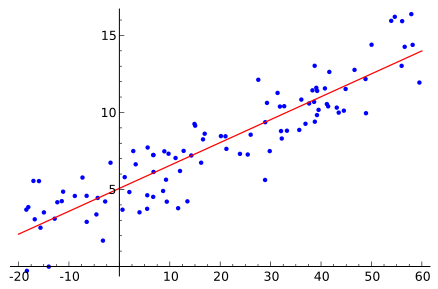
What is least squares? Intuitively, least squares finds the line deemed to best fit the data. Mathematically, least squares finds the line that minimizes the sum of the squared residuals. Note that when we say "line", it means "straight line". In Figure 1, the red line is the least squares line, the line that is considered to best fit the data.
|
| Figure 1 |
|
| Figure 2 |
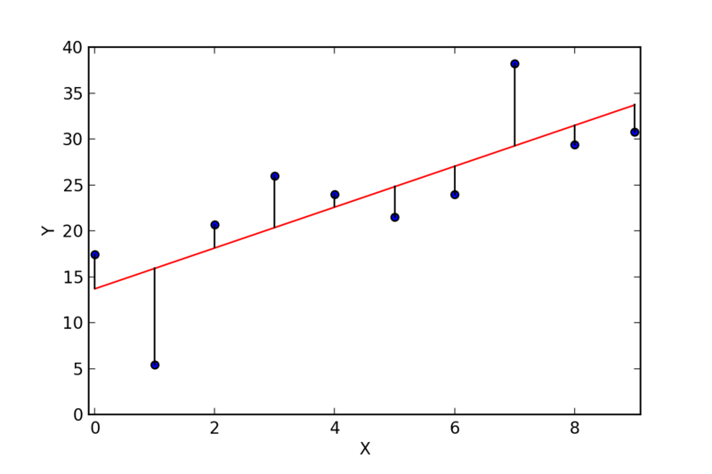
What is a "residual", as in "squared residual"? A residual is the difference between 1) the y value of a data point and 2) the y value in the least squares line. For example, in Figure 2, the dots are the data points, the red line is the least squares line, and the residuals are the lengths of the vertical lines. Residuals can be negative or positive.
What is "sum of squared residuals"? Referring to Figure 2, assume that the first data point is (0, 17.5), and that the least squares line includes the point (0, 14). The residual for the first data point is 3.5 (17.5 - 14). The squared residual is 12.25 (3.5 * 3.5). We do the same for each of the 10 data points, and sum the squared residuals. Squared residuals are always positive.
What are "slope" and "Y-intercept"? The least squares line is completely described by a slope and a Y-intercept. The slope is simply (change in y) / (change in x). The Y-intercept is the y value at X = 0. In Figure 2, the slope is (30 - 14) / (8 - 0) = 16 / 8 = 2, and the Y-intercept is 14.
Can I calculate a confidence interval for the slope? Yes. Since least squares is used to calculate a time trend, the analyst wants to know if the trend is significant. Rhe confidence interval (CI) for the slope, at some confidence level (eg, 95%), helps determine significance. If the CI includes 0, there is no significant trend. Otherwise, there is an upward (positive slope) or downward (negative slope) trend. However, as explained elsewhere on this web site, the confidence interval calculation is incorrect when the data points are based on few observations. Thus, a better method for determining the confidence interval of the slope is sought.
How is the least squares line calculated? The line could be iteratively determined, by drawing a line, calculating the sum of squared residuals, drawing another line, again calculating the sum of squared residuals, and repeating the process until the sum of squared residuals is minimized. Luckily, there is an exact method to calculate the line, without having to iterate through trial lines. Below, the exact method is shown in detail. We use a concrete example, with Texas mortality data, analyzing diabetes (E10-E14). Here are the data:
| Year | Year Index (X axis) |
Crude rate (per 100,000) (Y axis) |
Deaths |
|---|---|---|---|
| 2001 | 0 | 25.533 | 5445 |
| 2002 | 1 | 25.941 | 5650 |
| 2003 | 2 | 25.603 | 5663 |
| 2004 | 3 | 24.126 | 5426 |
The standard method for determining the Y-intercept, the slope, and CI of the slope is described in "Statistics", 2nd edition, by Murray Spiegel, pages 296 and 319. The method, as adapted for use within Vitalnet, is as follows:
First, define some terms:
· SS == sum of squares
· CL == confidence level
· SD == standard deviation
· YI == Y-intercept
· yrRngs == year ranges (4)
· df == degrees of freedom
· numer == numerator
· denom == denominator
Calculate preliminary values, to use later:
· yrRngs (number of year ranges) = 4
· sumX (sum of X values) = 0 + 1 + 2 + 3 = 6
· sumXX (SS of X values) = 0 + 1 + 4 + 9 = 14
· avgX (average X value) = 6 / 4 = 1.5
· avgXX (average X squared value) = 14 / 4 = 3.5
· df (degrees of freedom) = yrRngs - 2 = 2
· sumY (sum of Y values) = 25.533 + 25.941 +
25.603 + 24.126 = 101.203
· sumYY (SS for Y) = 651.934 + 672.936 +
655.514 + 582.064 = 2562.447
· sumXY (sum of XY values) = 0 + 25.941 +
51.206 + 72.378 = 149.525
· tVal (t Value) = 4.302656 (2 df and 95% CL)
· varX (variance of X vals) = avgXX - (avgX * avgX)
· varX = 3.5 - 2.25 = 1.250
· stdDevX (SD of X values) = sqrt (varX) = 1.118
Next, calculate the Y-intercept (YI):
· numer = (sumY * sumXX) - (sumX * sumXY)
· denom = (yrRngs * sumXX) - (sumX * sumX)
· YI = numer / denom
· numer = (101.203 * 14) - (6 * 149.525) = 519.692
· denom = (4 * 14) - (6 * 6) = 20
· YI = 519.692 / 20 = 25.985
Next, calculate the slope:
· numer = (yrRngs * sumXY) - (sumX * sumY)
· denom = (yrRngs * sumXX) - (sumX * sumX)
· slope = numer / denom
· numer = (4 * 149.525) - (6 * 101.203) = -9.118
· denom = (4 * 14) - (6 * 6) = 20
· slope = -9.118 / 20 = -0.456
Next, calculate confidence interval (CI) of slope:
· numer = sumYY - (YI * sumY) - (slope * sumXY)
· varOfEstimateOfYOnX = numer / yrRngs
· numer = 2562.447 - (25.985 * 101.203) -
(-0.456 * 149.525) = 0.870
· varOfEstimateOfYOnX = 0.870 / 4 = 0.218
· stdErrOfEstimateOfYOnX =
sqrt (varOfEstimateOfYOnX) = 0.466
· numer = tVal * stdErrOfEstimateOfYOnX
· denom = sqrt (df) * stdDevX
· halfInterval = numer / denom
· slopeLoLimit = slope - halfInterval
· slopeHiLimit = slope + halfInterval
· numer = 4.303 * 0.466 = 2.005
· denom = 1.414 * 1.118 = 1.581
· halfInterval = 2.005 / 1.581 = 1.268
· slopeLoLimit = -0.454 - 1.268 = -1.722
· slopeHiLimit = -0.454 + 1.268 = +0.814
· CI of the slope = -1.722 to +0.814
Finally, calculate coefficient of determination (r * r):
· numer = (yrRngs * sumXY) - (sumX * sumY)
· numer = (4 * 149.525) - (6 * 101.203) = -9.118
· xTerm = (yrRngs * sumXX) - (sumX * sumX)
· yTerm = (yrRngs * sumYY) - (sumY * sumY)
· xTerm = (4 * 14) - (6 * 6) = 20
· yTerm = (4 * 2562.447) - (101.203^2) = 7.741
· denom = xTerm * yTerm = 20 * 7.741 = 154.800
· co_of_determ = (numer * numer) / denom
· co_of_determ = (-9.118 * -9.118) / 154.800 = 0.537
The coefficient of determination (COD) is a measure of goodness of fit. If the data points fall on a straight line, the least squares line will be the same line, and COD = 1. If the data points are randomly distributed, COD = 0.
Vitalnet results for the above example. Some of the numbers may slightly differ, due to lower precision in the hand calculations.
In summary, the least squares finds the line considered to best fit the data, and determines if there is a significant upward or downward trend. However, as discussed elsewhere on this web site, the slope CI is incorrect when the data points are based on few observations. Thus, a better method for determining the slope CI is sought.